Direct Preference Optimization (DPO) for Diffusion Models

Chapter 1

What to teach after pretraining

Pretraining teaches a model the relationship between text and images. A prompt about a cat should produce a cat; a prompt about a city at night should produce a city at night. But that still leaves plenty of choices. One lighting setup looks professional, another looks flat. One texture is convincing, another looks plastic.

One caption: “A ginger cat on a wooden windowsill”

The caption fitsFlat lighting, blurry fur, awkward framing.

The caption fits here tooSoft lighting, detailed fur, careful composition.

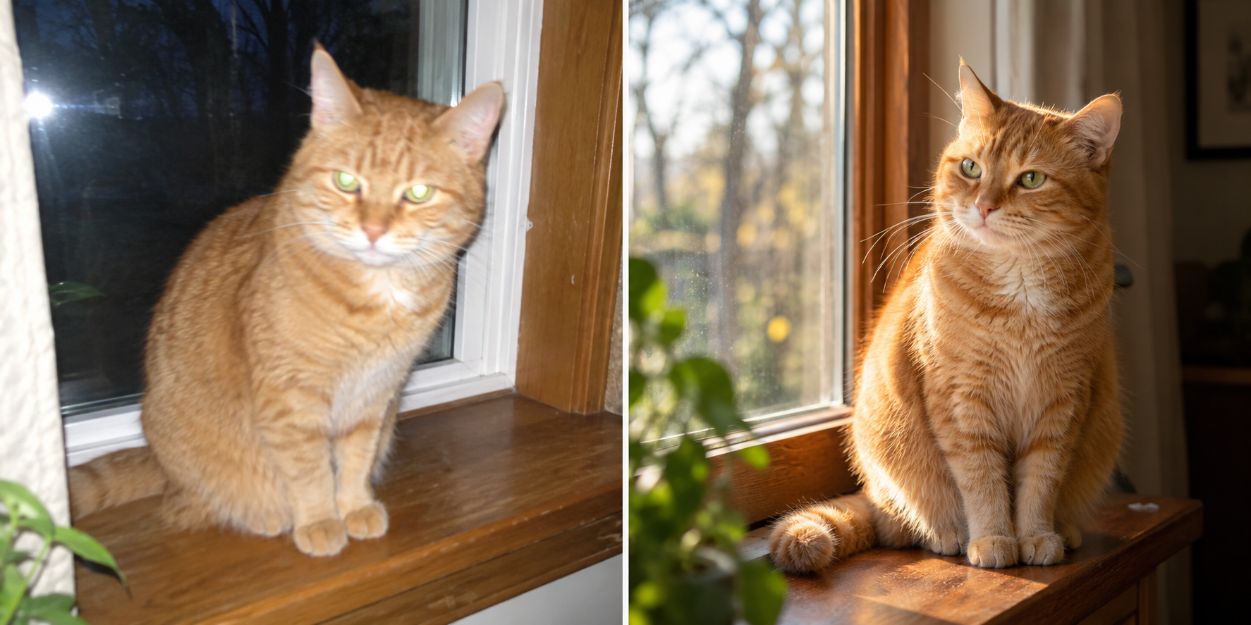
We still need to bring the model to the quality we want: it should produce the appealing image on the right more often than the flash photo on the left. An ordinary prompt does not explain this difference to the model: it fits both images. We need another training stage where we explicitly specify which results we prefer.

This is the task of preference optimization: teach the model to draw the cat with soft natural light more often than with harsh flash, spell text on signs correctly, include every object in the prompt, or draw hands without extra fingers.

We can provide this signal in two ways: choose the better result from a pair, or assign each result a numerical score. That choice determines how we train the model.

What is DPO? Learning from pairs

DPO (Direct Preference Optimization) is useful when we know which result we like but struggle to formalize that preference. We might want more pleasing light, natural skin texture, or a particular mood. How do we combine all of that into one score? Writing a metric or building a reward model that captures our taste can be difficult. What we really want is to optimize the vibe.

Choosing between two images is often easier than expressing a preference as a number: “this one looks right.” For a single prompt, we collect a pair: the selected image is the winner, and the other is the loser. DPO uses these comparisons to teach the model to favor the results we like.

One prompt: “A portrait of a woman at a table by a café window”

Loser · ordinary lightingEven, flat light makes the shot look mundane.

Winner · cinematicSide lighting, depth, and expressive shadows: this is the vibe we choose.

RL: learning from a score

In the second approach, the generator produces an image and a reward model returns a number: how well the result meets a chosen criterion. RL (reinforcement learning) uses these scores to update the generator toward higher expected reward. The model then generates new results, and the cycle repeats.

For example, we want to fix text in images. OCR reads the text on a sign; we compare it with the prompt and obtain a score. The generator gets a specific signal: a correct sign scores higher than one with a spelling error.

Prompt: “A café storefront with a sign reading CAFE”

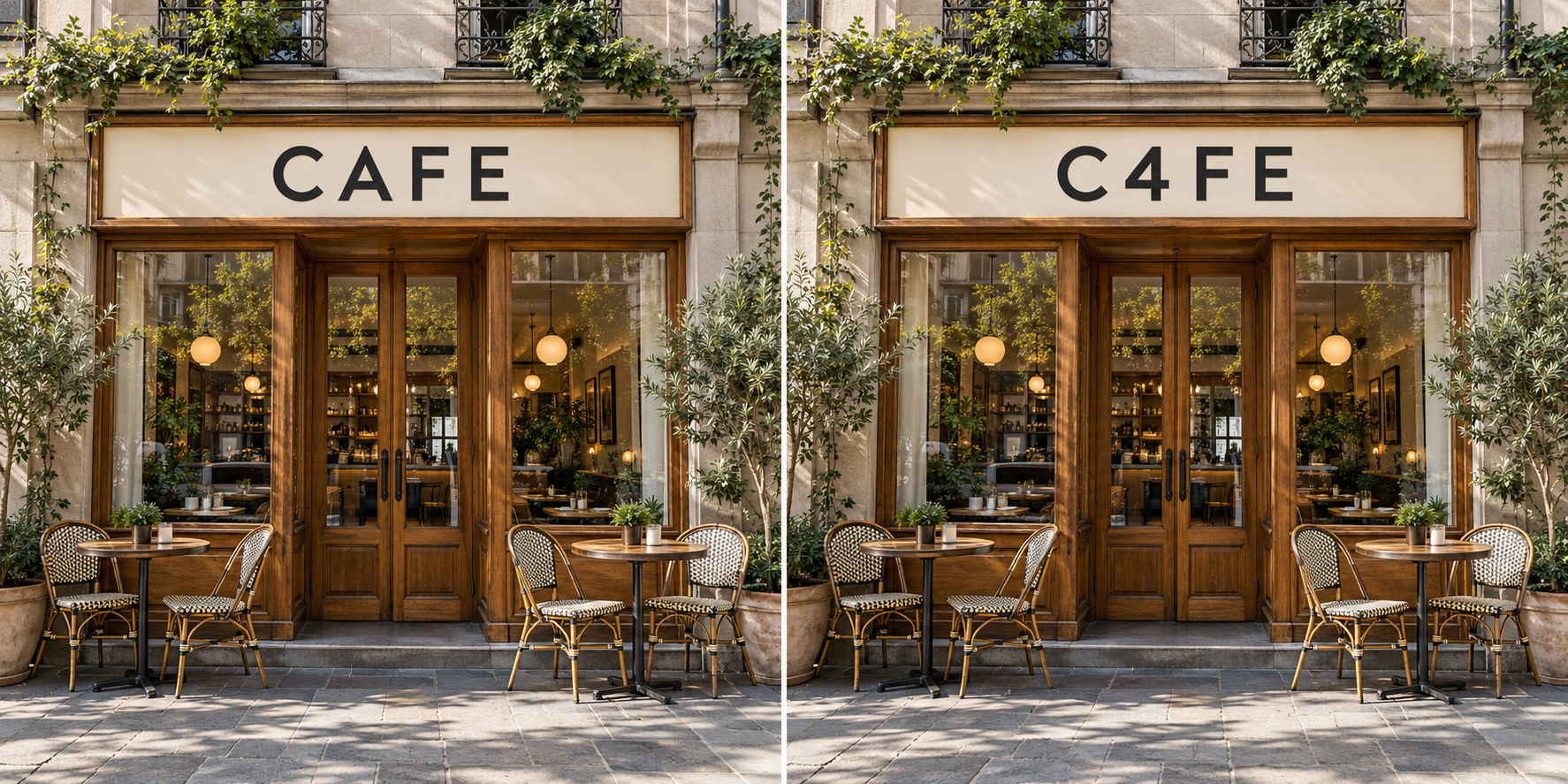
Image → OCR → scoreText: CAFE
4 / 4 characters → 1.00

Image → OCR → scoreText: C4FE
3 / 4 characters → 0.75

Chapter 2

The DPO loss: what DPO optimizes

For a prompt , we have two images: a preferred image and a rejected image . Define the model’s implicit reward as the log ratio of the image’s probability under the trainable model to its probability under the reference model:

Why use a probability ratio? We want to know how much more the trainable model favors an image compared with the original model. If its probability has increased, the ratio is above one and the logarithm is positive. If it has decreased, the logarithm is negative. The reference model provides a baseline for each image.

But the data contains no numerical reward: we only know that was preferred to . To connect reward to this label, we use the Bradley–Terry model of pairwise preferences. It gives the probability of choosing the winner as a sigmoid of the reward difference:

When the rewards are equal, the probability is ½. The higher the winner’s reward relative to the loser’s, the more confidently the model predicts that the winner will be chosen. This is an assumption about how preferences work, not a consequence of the pairwise label itself.

We now want the model to assign high probability to the observed choices. Minimizing the negative log of that probability over the dataset of pairs gives the DPO loss:

Inside the sigmoid is the difference between the winner and loser relative to the reference. We want the model to favor the winner more strongly. But the function only sees the difference. It does not require each step to improve the winner’s absolute quality. We will return to this limitation.

Adapting this to diffusion

In a language model, we can compute the probability of a given sequence from token probabilities. A diffusion model produces an image through a denoising process, so plugging its likelihood directly into the same formula is harder.

To adapt DPO to diffusion models, we use a variational bound, as in Diffusion-DPO. The loss can then be written in terms of noise prediction errors on the winner and loser. First, define the differences between those errors for the trainable and reference models:

The resulting loss is:

Recall the two portraits: one with ordinary lighting, the other with cinematic lighting. During pretraining, the model learned to reconstruct both images from noise. Now we tell it: “for the same prompt, we want the second version more often.” DPO changes training to favor reconstructing the image with cinematic lighting over the one with flat lighting. Across many such pairs, the model can pick up our lighting preference even though we never wrote down what makes the light beautiful.

Here is how this training changes generated images. Below are SDXL results before and after Diffusion-DPO, using the same prompts.

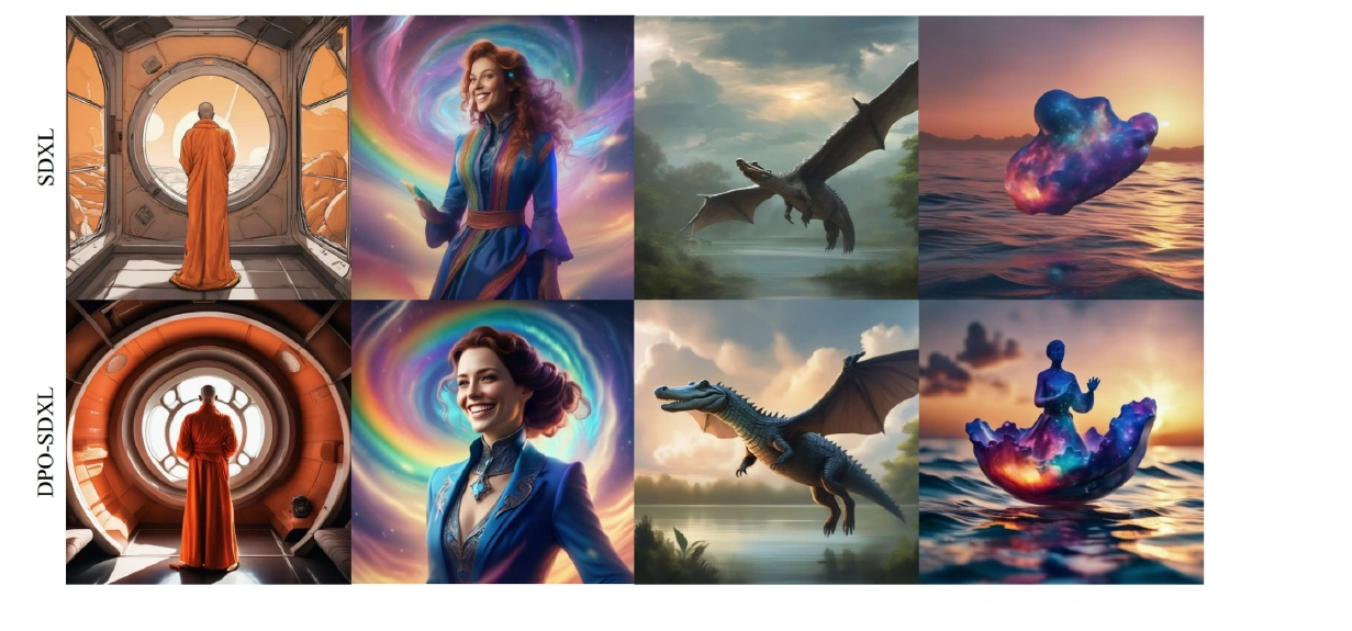
Each pair changes in a different way:

• The monk. In the original image, the room looks like an illustration with flat fills. After DPO, there are deep shadows, highlights on the round frame, and more pronounced folds in the clothing. The scene has more depth.
• The portrait. Instead of a waist-up figure with a small face, we get a closer portrait. Facial features, strands of hair, and the trim on the blue outfit are easier to see; the face stands out more against the colorful swirl.
• The dragon. In the top row, it is almost entirely in shadow. In the bottom row, it is larger and better lit: the scales on its neck, the ridge along its back, and its wing membranes are visible.
• The scene above water. A shapeless glowing object becomes a human figure on a bowl-like form. The colored glow reflects in the water. Here, the structure of the object itself changes, not just its lighting or texture.

This is the practical value of DPO: selecting images can convey a preference for lighting with more depth, finer detail, and more expressive presentation, without a separate formula for each quality.

What to do with β

Our loss contains a parameter that multiplies the error difference before the sigmoid:

β scales the error difference between the winner and loser before the sigmoid. With a large β, even a small advantage for the winner can push the sigmoid close to one: the pair already looks confidently separated, and its training signal weakens. With a smaller β, saturation requires a larger advantage.

In practice, β is tuned together with the learning rate. If the signal from pairs fades too quickly, the model does not get enough time to learn from the data and absorb the preference. We need to give it time to learn instead of pushing the loss into saturation immediately. The balance is between how fast the model changes and how fast the chosen β weakens the signal.

Chapter 3

Which pairs are actually useful?

Training needs winners and losers. But which images should go into these pairs so that the model learns the preference we want?

FiFA: margin, prompt quality, diversity

The most frustrating case in pairwise training is a dataset full of uncertain winners. One annotator preferred the lighting, another the composition, and a third simply chose a different style. Collecting many such pairs does not necessarily remove the uncertainty.

The score difference between the winner and loser is called the preference margin. If an evaluator barely distinguishes the images, the margin is small; if it confidently favors one, the margin is large. You can see this in the cat-knight and dragon examples: both images in the low-margin pairs look acceptable, while one image in each high-margin pair clearly violates the prompt.

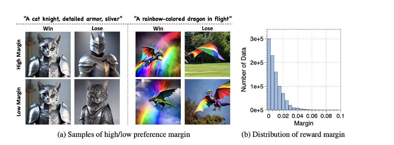
This is the basis of selection in FiFA. The method considers three things: how clearly the winner beats the loser, how well the prompt is written, and how diverse the prompts in the selected set are. Pairs are ranked by a combined score.

In my own work, I read these three components as follows. First, it should be clear why the winner is better. Second, the prompt should let us judge the result: the word “cat” tells us little about what was expected. Third, the selected examples should cover the domains we need. If all strong pairs are portraits, we cannot automatically expect the same improvement in other scenes.

This does not mean a long prompt is always better than a short one. Detail helps when it makes the selection criterion clearer. Lots of words without a clear request do not create a useful preference signal.

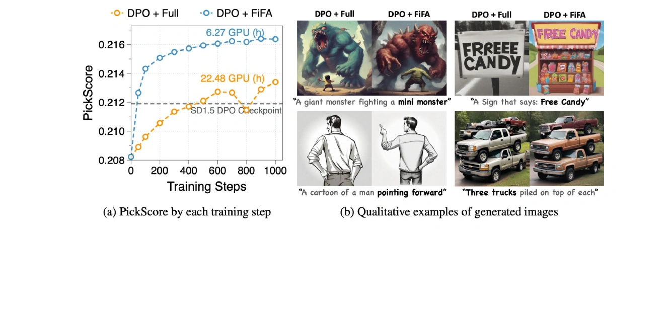
My takeaway is to establish a clear signal in each pair before scaling up the dataset. More ambiguous comparisons do not necessarily mean more useful learning.

I usually collect data in several rounds: start with automatic or synthetic labels, then generate new examples with the improved model and send them to human annotators.

Human annotation is expensive primarily because of the organization it takes. You need to agree on criteria, explain them to annotators, and check consistency. If you need professional judgment, it is hard to replace a person with the average of many random votes.

So I would first select pairs where the reason for the choice is already clear. A reward model can help with this selection, leaving ambiguous cases for human review.

What if both images are good?

Suppose two bad images have a large margin, while two excellent images have a small one. Would we really choose the first pair just because it is easier to distinguish?

No: a large margin is no substitute for a good winner. We want both a strong positive example and a clear difference from the negative one. If the winner itself is poor, we have chosen a poor target for the model.

And two excellent images do not have to compete. If both work for us, we can train the model to reconstruct each one without a loser term: use them for SFT. Here we select good examples on their own merits rather than trying to find the worse image in every pair.

My starting recommendation is simpler: first get a good winner and a clearly worse loser. I would add complex rules for ambiguous pairs after that baseline works.

Can we use another model’s images?

Off-policy data is one of DPO’s convenient features. Pairs can be collected in advance; not every example has to come from the current checkpoint. We can also use pairs from different generators: a stronger model provides the winner, and a weaker one the loser.

This can provide a clear signal without a complex evaluation system. But along with quality, we transfer the generator’s character: lighting, saturation, and textures. So resemblance to the teacher model does not, by itself, prove that we learned the intended preference.

There is also a separate question about negatives. If the loser is so far from the current distribution that our model almost never produces anything similar, how useful is it to push away from it? I do not have a universal answer. My experience with a weaker and a stronger model was positive, but that does not imply that worse losers always mean better training. An external winner paired with an on-policy loser remains a separate hypothesis to test.

Chapter 4

The loss improves, the images get worse

The DPO loss asks the model to reconstruct the winner better relative to the loser. But this comparison can improve even if winner reconstruction gets worse: loser reconstruction only has to deteriorate faster. The winner’s relative advantage grows, so the DPO loss falls, even as errors on both images rise.

The plot from Diffusion-SDPO shows changes in error relative to the reference. Orange is the winner; green is the loser. Both rise: the model reconstructs both images worse. But the loser error rises faster, so the “winner − loser” difference, shown in purple, falls. For DPO, that difference is moving in the desired direction even though winner reconstruction is deteriorating.

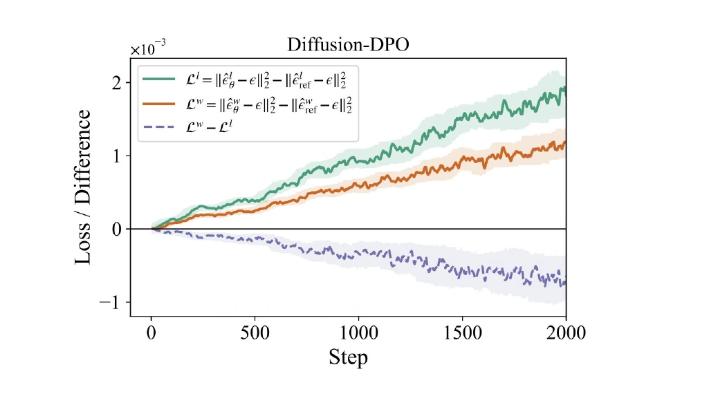
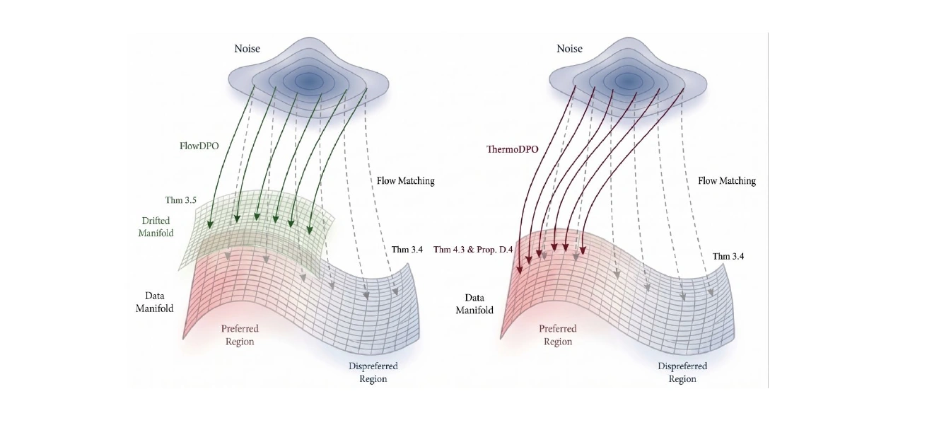
In generated images, this might look like the model picking up the desired cinematic lighting while faces and hands become distorted. It has learned the lighting preference, but its ability to draw plausible objects has deteriorated. This is an example of manifold drift: in chasing a preference, the model loses its ability to generate images properly.

Chapter 5

Keeping the model close to good examples

A common strategy is, in effect, to do SFT on the winner alongside DPO. I would highlight three methods that I find useful in practice: DPO + SFT, BDPO, and ThermoDPO.

SFT on the winner

The most direct approach is to add the standard training loss on the winner to the DPO loss:

The model must also learn to reconstruct the winner, so that the loss does not decrease solely by making the loser worse.

BDPO: bounding the loser term

SFT directly increases the probability of a good example. Bounded-DPO, proposed for language models, puts more emphasis on learning from the winner in a different way: it limits how much the loss can decrease through loser suppression alone.

In ordinary DPO, the model can improve the winner-to-loser probability ratio by driving the loser’s probability lower and lower. BDPO replaces the loser probability with a mixture: part comes from the trainable model and part from the frozen reference. Even if the trainable model assigns the loser almost zero probability, the reference contribution remains. Further reducing the loser’s probability therefore becomes less and less useful.

Once further loser suppression barely helps, reducing the loss requires increasing the winner’s probability. This is the connection between BDPO and SFT: training puts more emphasis on the good example, even though no separate SFT loss is added.

ThermoDPO: anchoring to the winner

In ThermoDPO for flow models, the connection to SFT is more direct: one loss combines pairwise comparison with the ordinary task of reconstructing the winner. While the preference is not yet learned, the model learns to distinguish the winner from the loser. When the pairwise comparison provides little signal, training on the winner continues: the same task we previously added through SFT regularization.

To write the loss, define three quantities. increases when the winner error decreases relative to the reference; works the same way for the loser. is computed from the reference and does not change as the model is updated:

Here are the differences in flow-matching error between the trainable and reference models, is the reference error on the winner, and is the temperature. To reduce the loss, we need to increase the winner’s share of this fraction.

Once the winner confidently beats the loser, making the loser worse does almost nothing to reduce the loss. The model continues learning to reconstruct the winner itself: a learned preference alone is no longer enough.

In the toy experiment below, this is visible in the front view, the second plot. The green points from ordinary DPO form an arc above the original surface: the model has shifted its generations but moved off the manifold. The red ThermoDPO points remain closer to the original shape. This separates the preference shift from how well the data geometry is preserved.

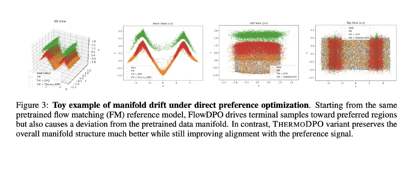
The practical purpose of this regularization is to learn the desired lighting or style while continuing to learn to reconstruct good images. An advantage over the loser alone is not enough.

Chapter 6

Where I would use DPO

When to choose DPO

I would use DPO where a preference is easier to show than to express through a reward: which lighting looks professional, which composition works better, which style we want. Pairs let us convey these choices to the model even without a separate reward for them.

For a specific task, such as fixing illegible text, I would look toward RL with a reward for that task. We can evaluate whether the text is spelled correctly and train the model to improve that particular result. The constraints are the evaluator’s quality and how many rollouts we can afford.

Where to get good examples

The choice of winner largely determines the result. If we take good images from another generator, we may inherit its characteristic lighting and style along with its quality. Even the CFG used to produce the examples affects what we teach the model. When collecting pairs, we therefore need to understand which properties of the winner we actually want in our own generations.

The source of good examples also determines whether we need a separate SFT stage before DPO. If good external examples are already available, we can use them as winners and train with DPO and SFT together. If we collect pairs from our own generations, preliminary SFT can improve the material for the next round: the model will produce better winner candidates.

How to continue training

DPO can run for several rounds: start with automatic labels, then, after the model improves, collect new pairs and send them to human annotators. The next round will then use generations from the updated model.

After DPO, we can move to RL: first use pairs to establish broad visual preferences, then use a reward to address specific weaknesses.